When operated as a random scan display unit, a CRT has the electron bim directed only to the parts of the scan where a picture is to be drawn. Random scan monitors drown pictures one line at a time, also called vector display.

The refresh rate on a random scan display depends on the number of lines to display picture definition in a row stored as a set of line drawing commands in an area of memory. Random scan systems are designed for line drawing applications and can’t display realistic shaded scenes. Since a picture definition is stored as a set of line drawing instructions and not as a set of intercity values for all pixels.

The architecture of random scan or vector scand display.

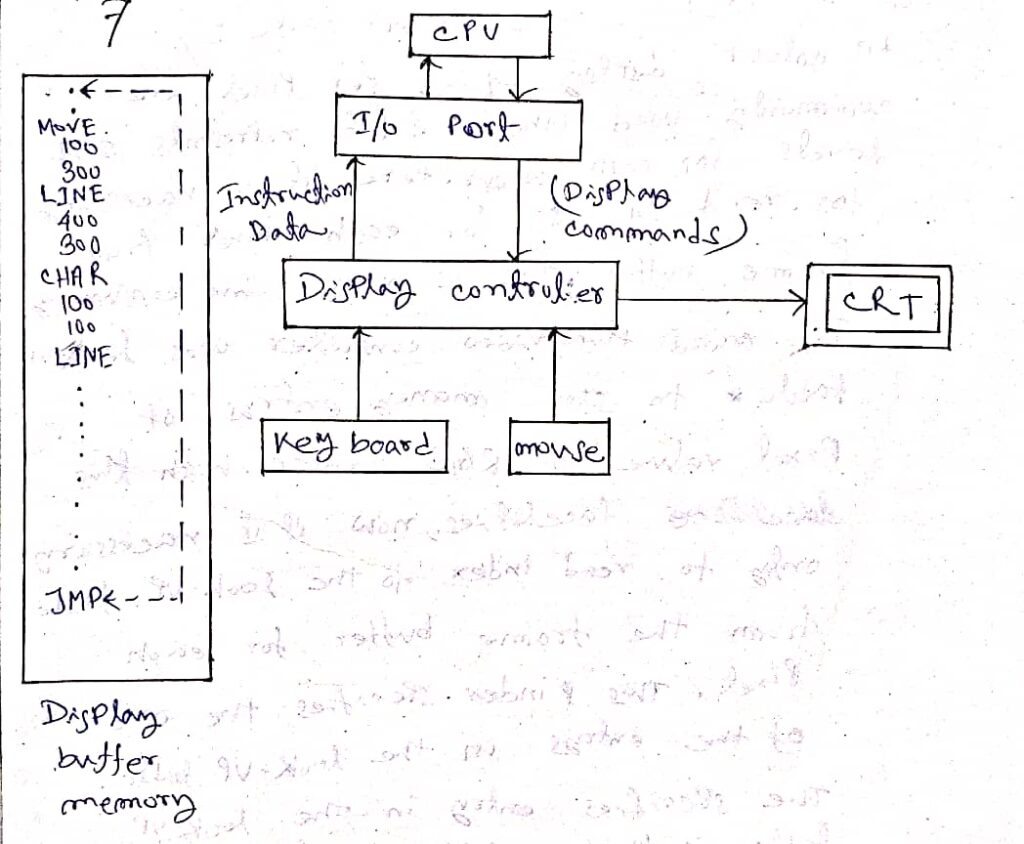
The figure shows the tropical vector display architecture consisting of a display controller CPU, display buffer memory, and CRT. A display controller connector as an I/O peripheral to the CPU. The display buffer memory stores to the computer-produced display list or display program.

The display controller interprets commands for floating point lines and characters and sends digital coordinates to a vector generator. The vector generator then converts the digital coordinate values to analog voltages for a beam deflection circuit that displays an electron beam writing on CRT phosphor coating.

Color table or Look-up table.

In color display, 24 bits per pixel are commonly used where 8 bits represent 254 levels for each color. Here it is necessary to read 24 bits for each pixel from the frame buffer. This is very time-consuming to avoid this, so the video controller uses a look-up table to store many entries of pixel values in RGB format with this facility, now it is necessary only to read the index to the look-up table from the frame buffer for each pixel.

This index specifies one of the entries in the look-up table. the specified entry in the look-up table is then used to control the intercity or color of the CRT.

Grayscale:

grayscale with a monitor that has no color capabilities, color functions can be used in an application program to set the grass scale for displayed primitive. Newmatric values over the range from 0 to 1 can be used to specify gray scale levels, which are then converted to appropriate binary code for storage in the Rasten display system.

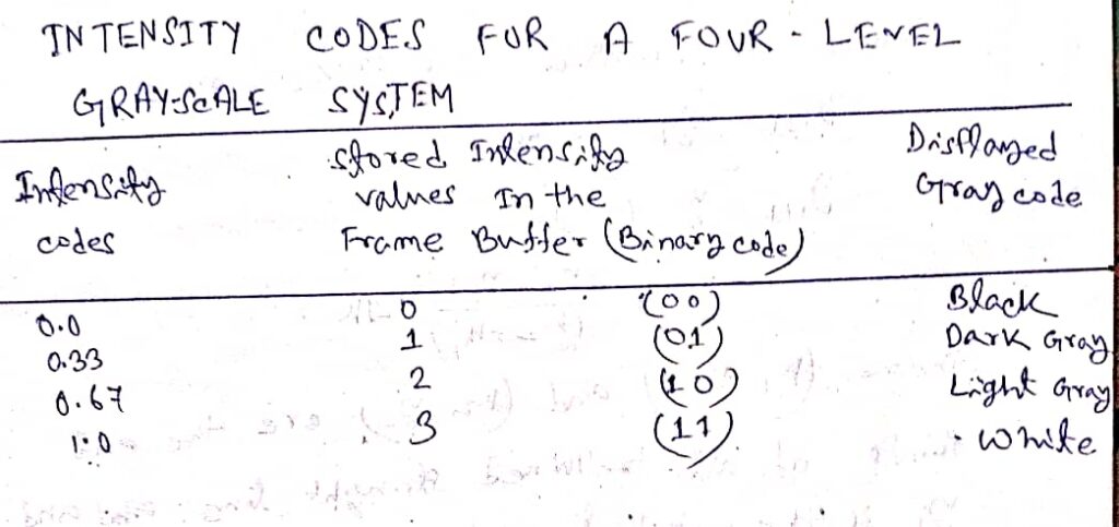
In this example, any intensity input value near 0.33 would be stored as the binary value 01 in the frame buffer and displayed as dark gray.

Line drawing Algorithm:

Considering the assumptions most line-drawing algorithms used incremental methods. In this method, the line starts with the starting point. Then a fixed increment is added to the current point to get the next point on the line. This is continued till the end of the line.

Digital Differential Analyzer(DDA):

One technique for obtaining a rasterized straight line is to solve the governing differential equation for a straight line.

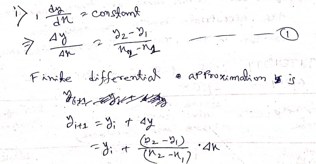
Where (x1, y1) and (x2, y2) are the endpoints of all required straight lines and y_i is the initial value for any given step along the line.

In fact equation

1. Represent a recursive relation for successive points in a line, it is called DDA[Digital Differential Analyzer]

Digital Differential Analyzer routine for rasterizing a line:

The line end point are (x1, y1) and (x2, y2) assumed not equal. integer is the integer function(The algorithm assumes integer functions are floor functions).

Sign return -1, 0, 1 for arguments <0, =0, >0 respectively approximate the line length.

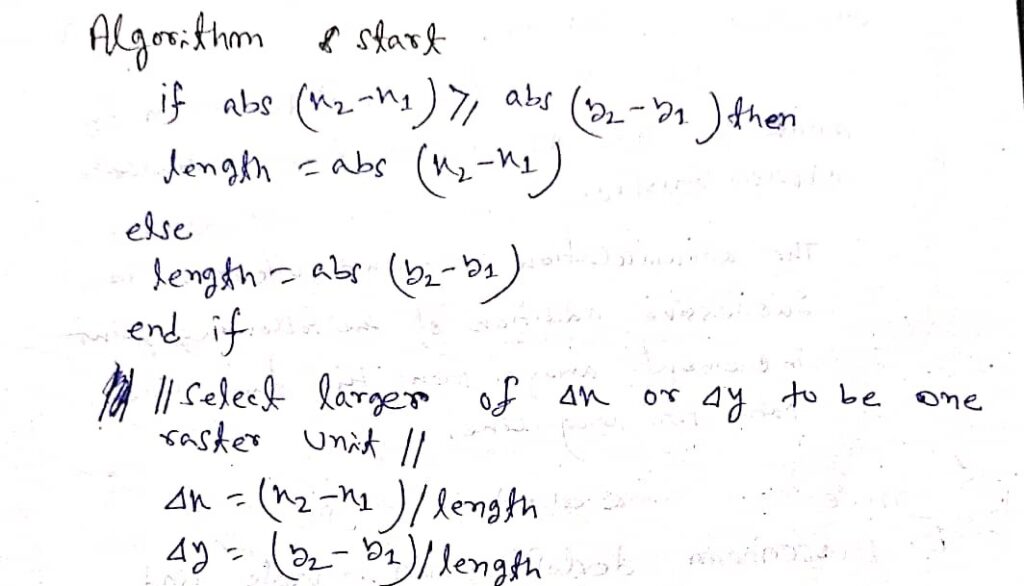
Round the values rather than truncated so that center pixel addressing is handled correctly.

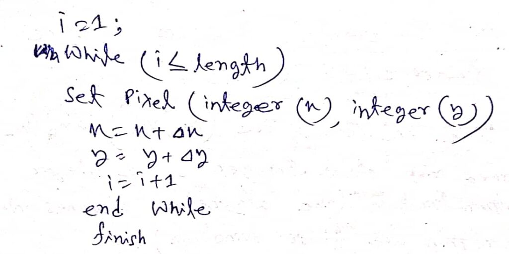
The DDA algorithm is a faster method for calculating pixel positions than the actual method employed by directly using the equation y=mx+c.

It eliminates multiplication by making use of raster characteristics. the accumulation of round offeror in successive addition of the following point increment away from the true line path for the long line.

Bresenham line drawing Algorithm:

Bresenham developed an accurate and efficient rasters line generating algorithm. The algorithm always increments by one unit in either x or y. Depending on the slope of the line. The increment in the other variable either ‘0’ or ‘1’, is determined by examining the distance between the actual line and the nearest grids location. This distance is called the error. the algorithm is efficiently constructed 80 that the sign of the error term needs to be examined.

General Bresenham algorithm:

A full implementation of the general Bresenham algorithm requires modification for line lines in other options. Bresenham algorithm is generalized to lines with arbitrary slopes by considering the symmetries between various actors and coordinates of the xy plane.

For a line with (+) slope greater than one, we interchange the x and y direction. If the initial position for the line with (+) slope is the right-hand point, both x and y decrease as we step from right to left.

For (-) slopes the procedures are similar except that now one coordinate decreases as the other increases.

Bresenhem circle drawing algorithm:

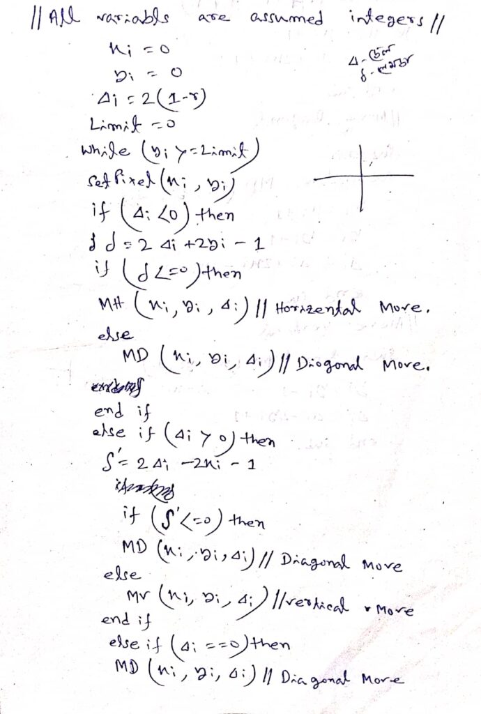
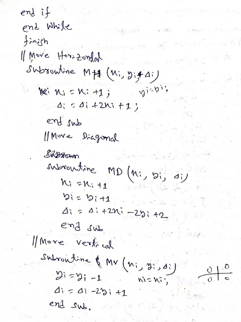
One of the most efficient and easiest ways to derive a circle is the presented Algorithm to begin with only one octant of the circle needs to be generated. The other parts of the circle are obtained by successive reference. Assuming a clockwise generalizal of the circle there are three possible selections for the next pixel which represents the circle.

Horizontally to the right, diagonally, and downward. These are levels AMW, MV, and MD respectively. The algorithm chooses the pixel which minimizes the square of the distance between one of these pixels. Bresenhem’s incremental circle generation algorithm for the first quadrant.

Explain Translation & Rotation:

Translation:

A translation is applied to an object by repositioning it along a straight-line path from one coordinate location to another position. We translate a two-dimensional point by adding translation distances T_x and T_y to the original point to a new position (x^I, y^I)

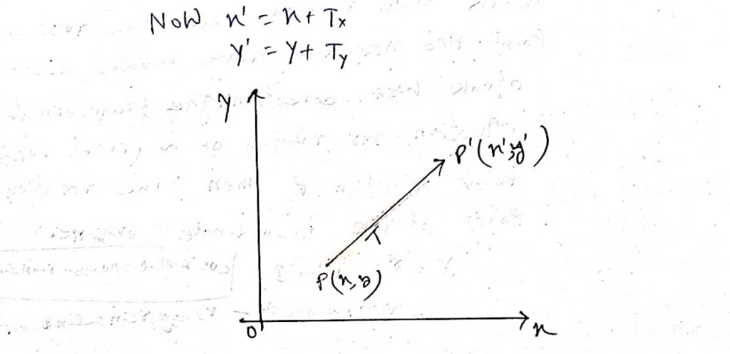
We can express the translation equation by using a signal matrix equation as below.

This allows us to write two-dimensional translation equations in a matrix form

p^I=p+t

Rotation:

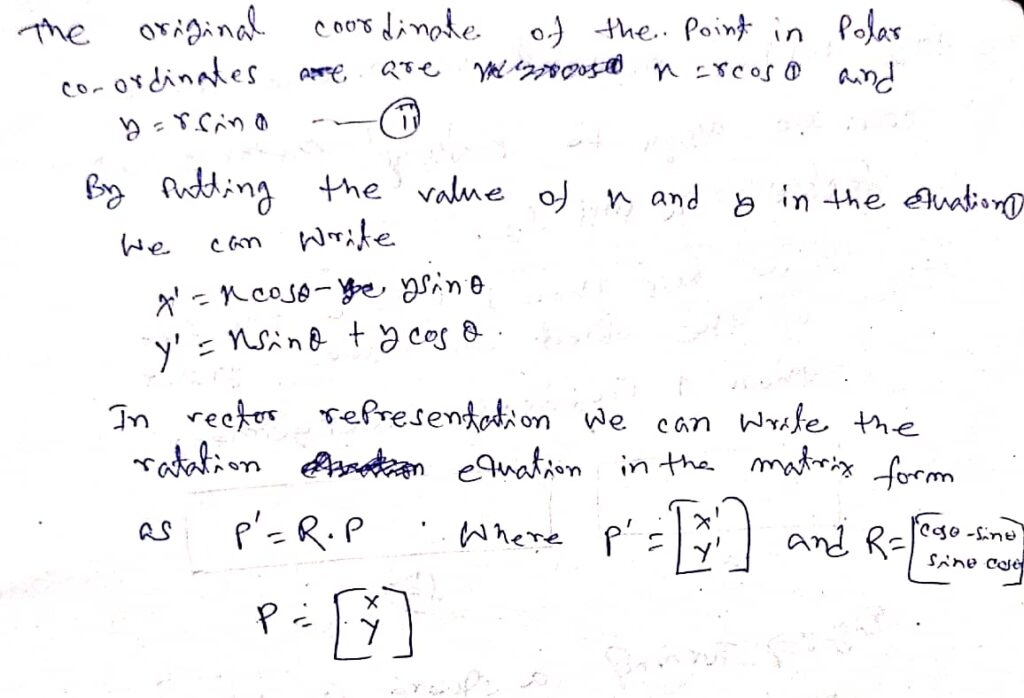
The two-dimensional rotation is applied to an object by repositioning it along a circular path in the xy plane to generate a rotation we specify a rotation angle Q and the position(xr, yr) of the rotation point about which the object is to be related. A positive value for the rotation angle defines counterclockwise rotation about the rotation point and a negative value rotates objects clockwise direction.

The transformation equation for rotation of a (pixel position) point position p, when the rotation point is at the coordinate origin.

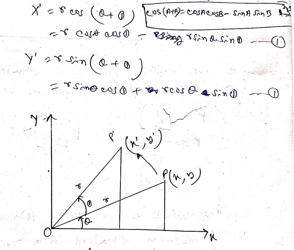
Here r is the constant distance of the point from the origin. Angle (Pai) is the original angular position of the point from the horizontal axis and Q is the rotation angle.